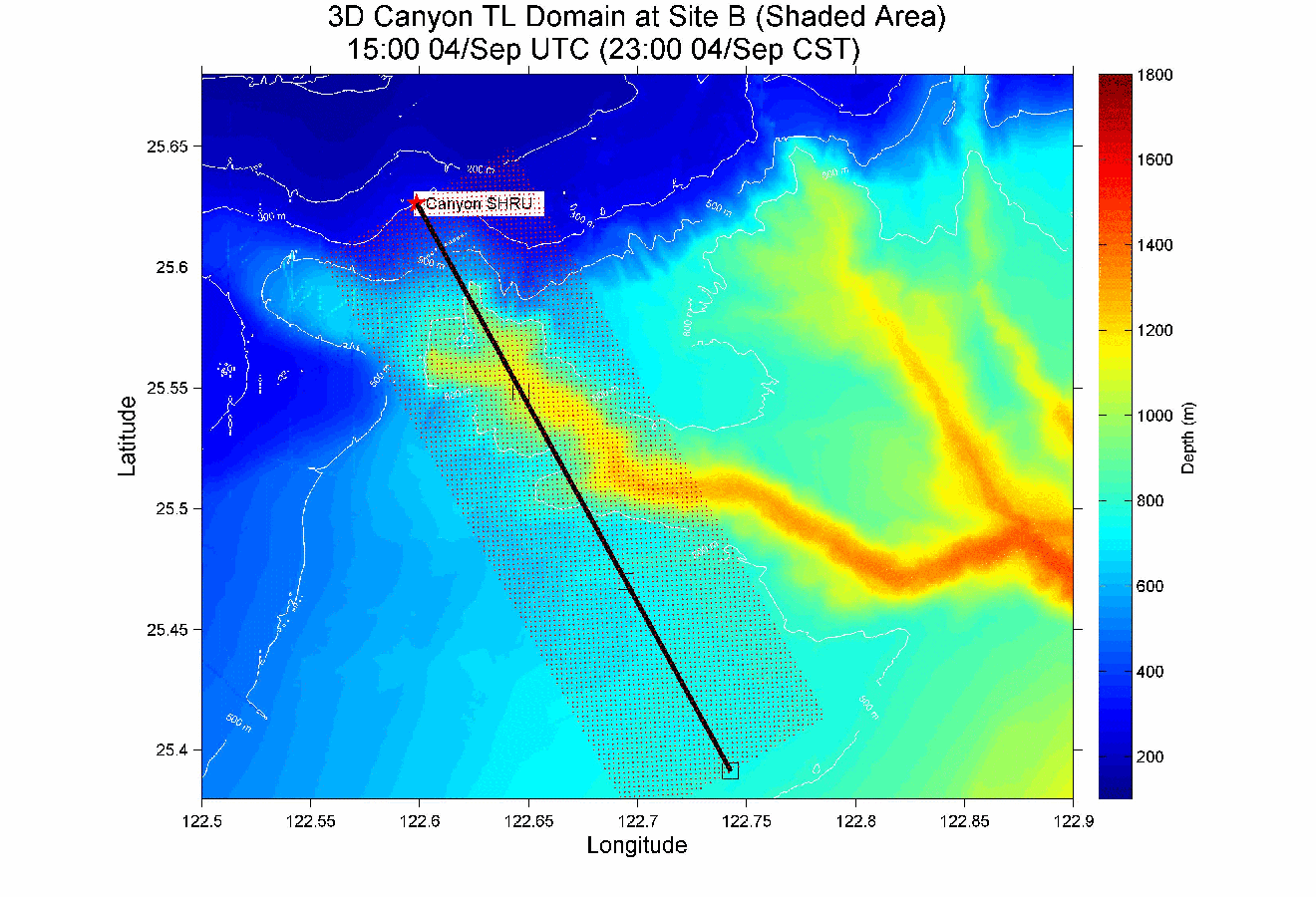
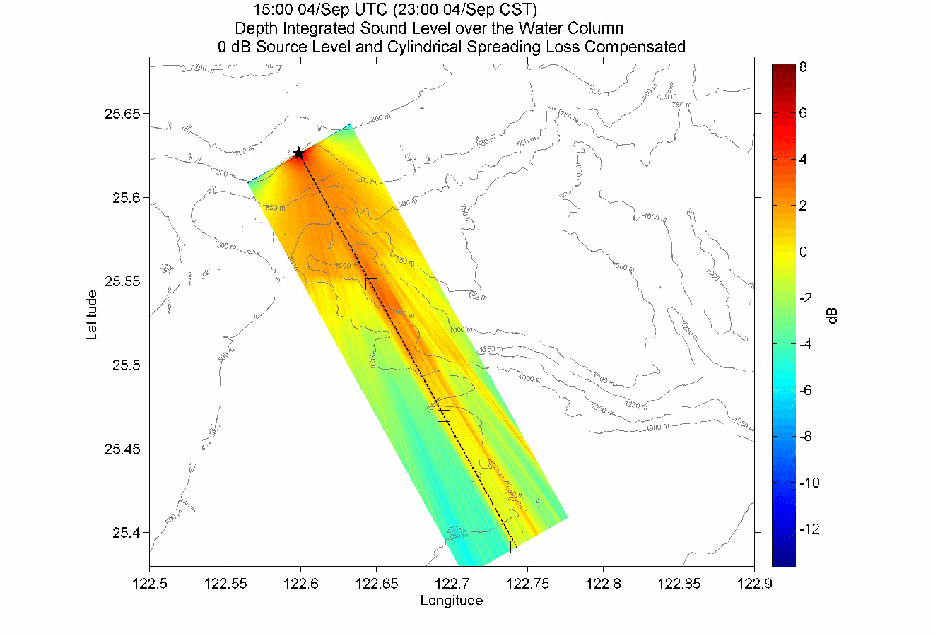
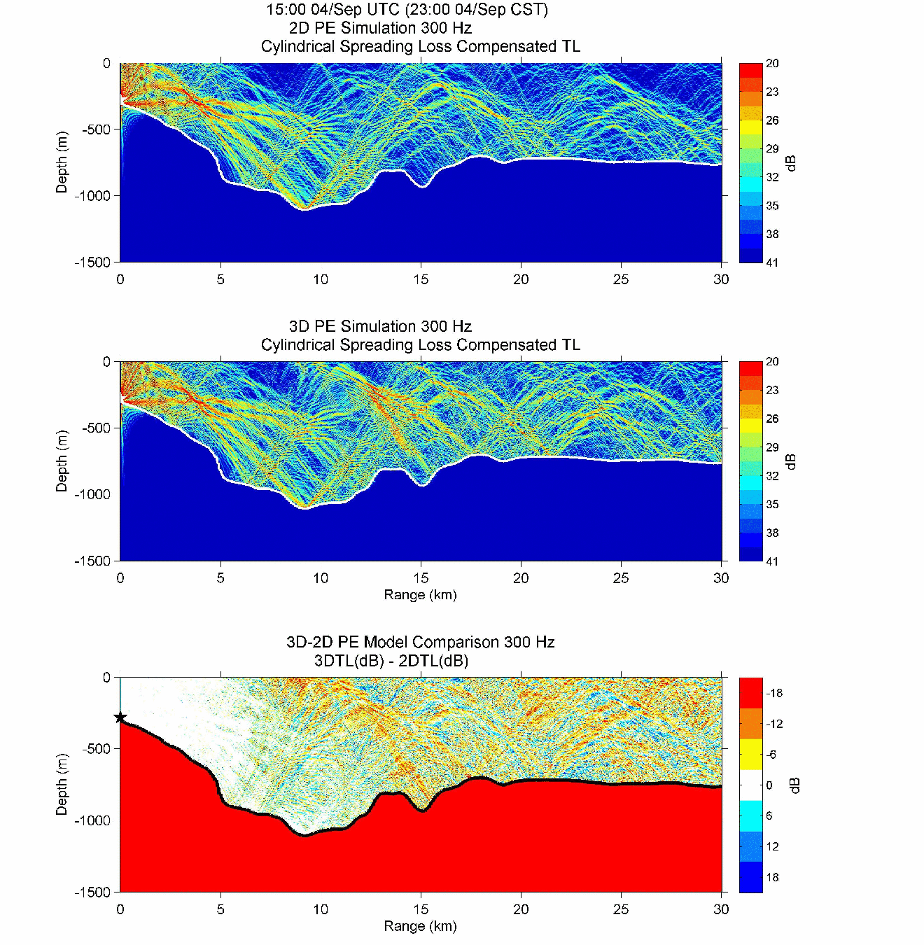
| Sep 04 1500Z (Sep 04 2300CST): Snapshot of the Estimated Propagating Sound Field over the North Mien-Hua Canyon | ||||||
|---|---|---|---|---|---|---|
| Click on any picture icon for a full resolution plot | ||||||
|
PE source location:  25 38.993 N 122 36.014 E (Canyon SHRU deployed location on QPE IOP Leg 1, water depth 200 m); PE source frequency: 300 Hz
x-y-z convention: PE marching direction (x), transverse direction (y) and depth (z); Step sizes: dx = 20 m, dy = 1.25 m, dz = 0.833 m
Water column: Real-time MIT MSEAS system (4.5 km resolution); Bathymetry: UNH 100 m resolution data
Bottom: General sandy bottom (sound speed 1,700 m/s, density 1.5 g/cm3, attenuation coef. 0.5 dB/λ)
The four-dimensional ocean utilized for this work is produced by the Multidisciplinary Simulation, Estimation, and Assimilation System (MSEAS). The physical fields associated with these acoustics results are found here. The three-dimensional MSEAS acoustical products are found here.
This forecast is for predicting the 3-D canyon acoustic effect on sound propagation and also the temporal variability of the sound field due to water-column condition changes. The model is an acoustic propagation program that employs the split-step Fourier (SSF) technique to solve the 3-D parabolic acoustic wave equation (PE) for one-way propagating waves in a Cartesian coordinate system. Bottom density contrast and volume absorption have been taken into account, and the PE starter is a 3-D variant of the Thomsons wide angle starter. Most importantly, the PE approximation is made with the 3-D version of the Thompson-Chapman wide angle expansion. The initial program development efforts are made by J. Colosi of NPS, USA, and the later modification for the Thompson-Chapman wide angle PE is done by T. Duda of WHOI. The 3-D wide angle starter and the treatment on bottom density are added by Y.-T. Lin of WHOI. This work is sponsored by the ONR.
| Sep 04 1500Z (Sep 04 2300CST): Snapshot of the Estimated Propagating Sound Field over the North Mien-Hua Canyon | ||||||
|---|---|---|---|---|---|---|
| Click on any picture icon for a full resolution plot | ||||||
|
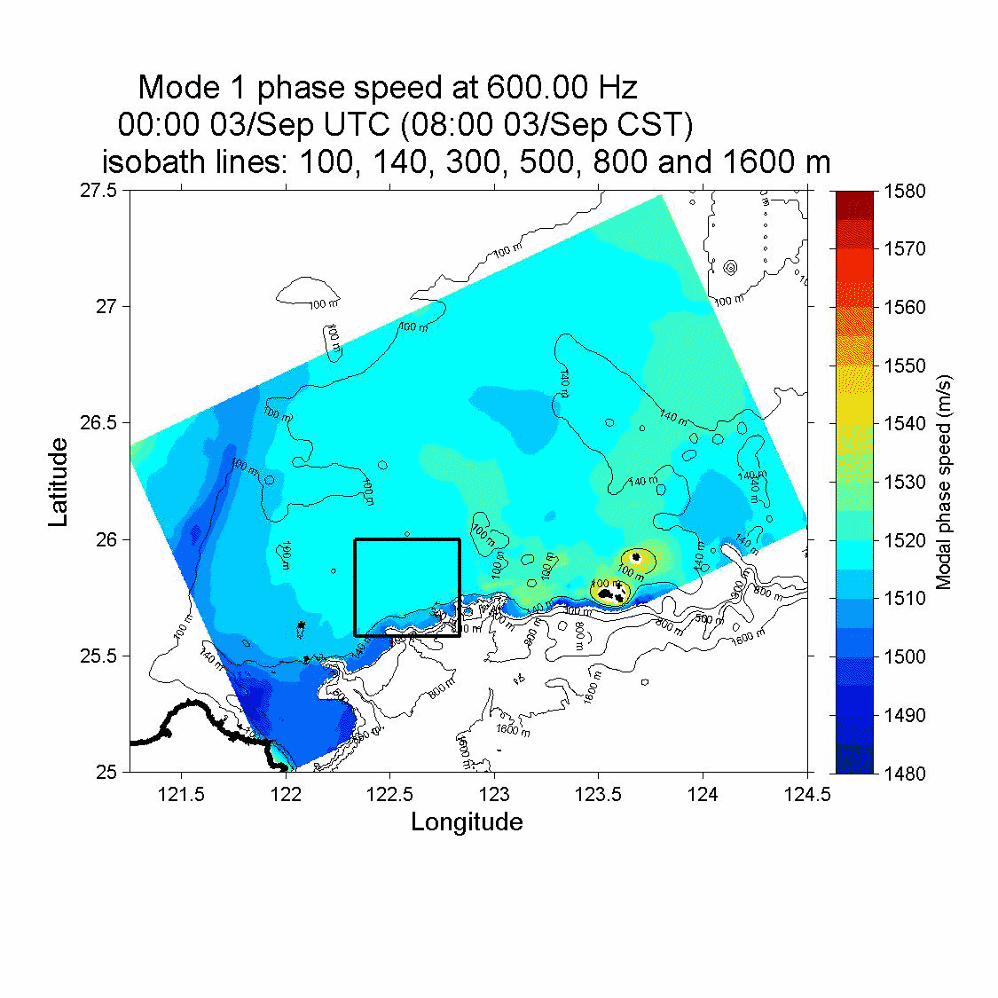
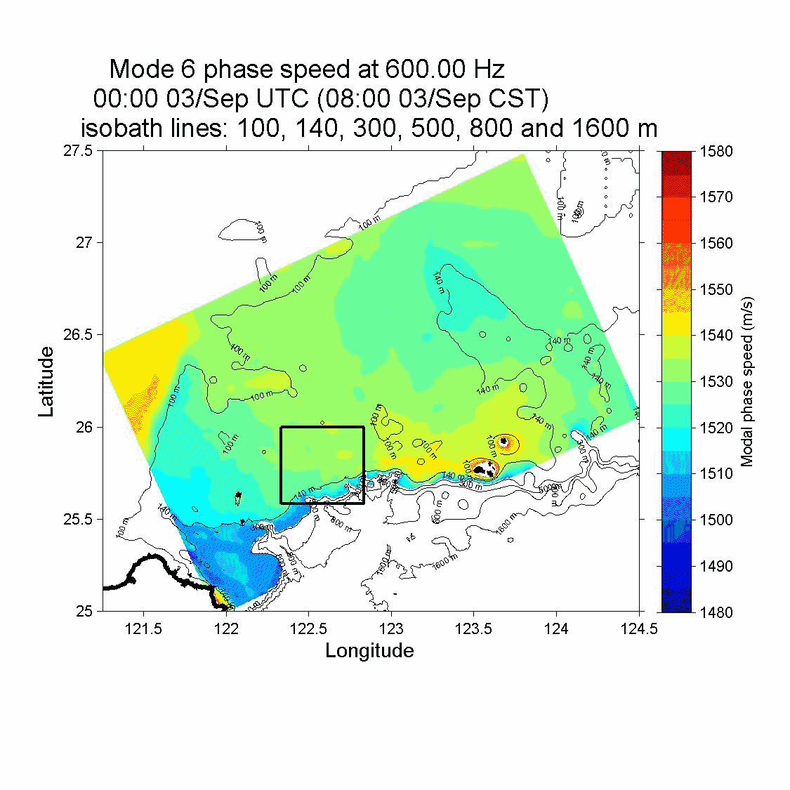
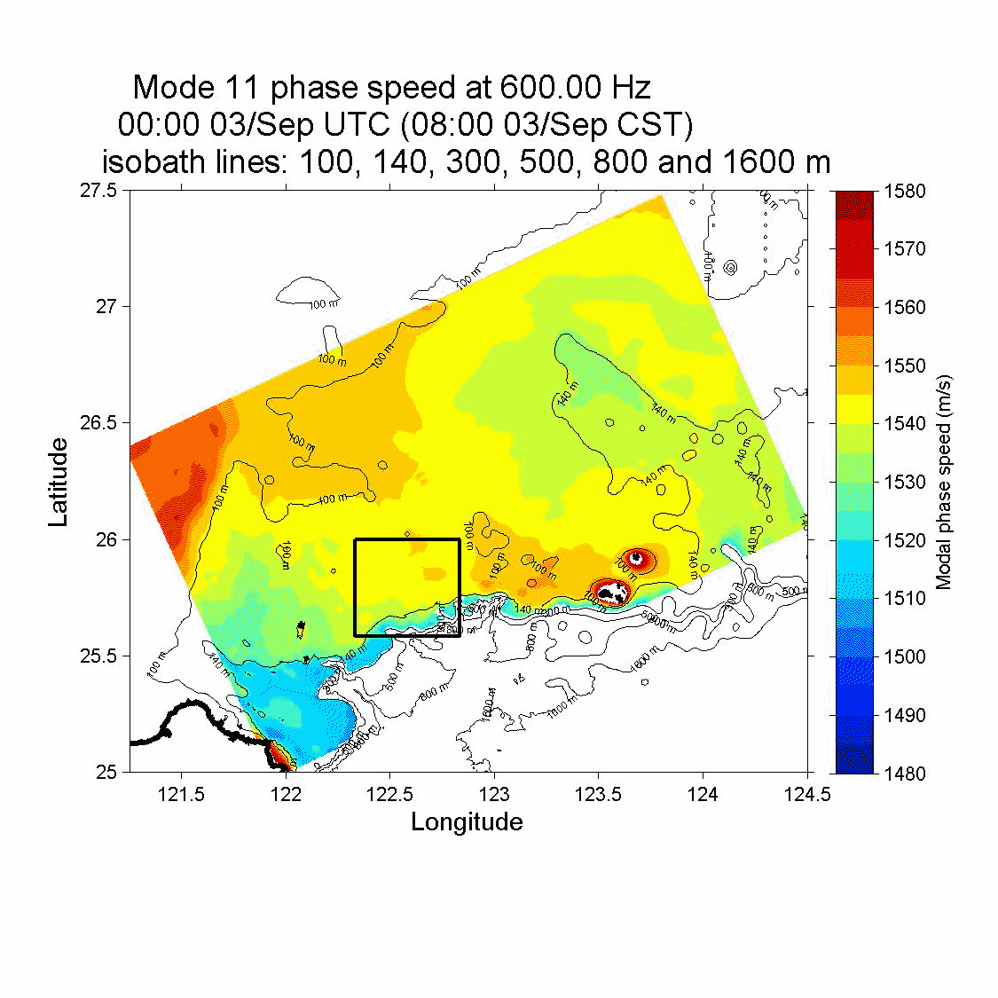
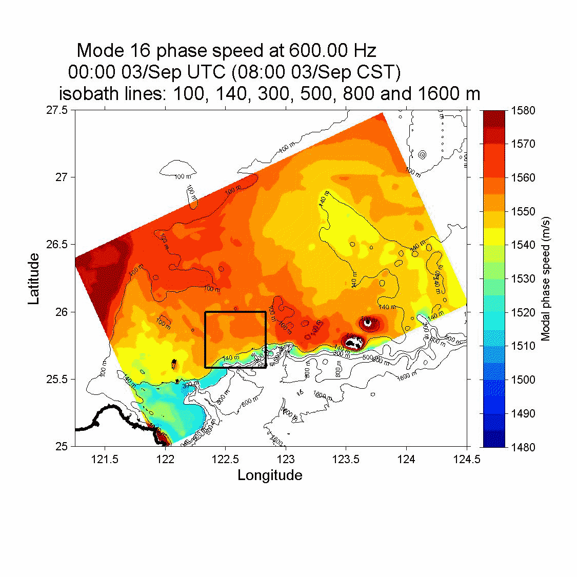
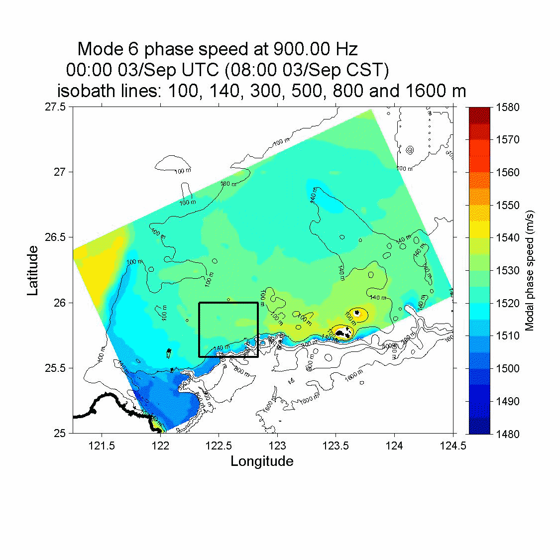
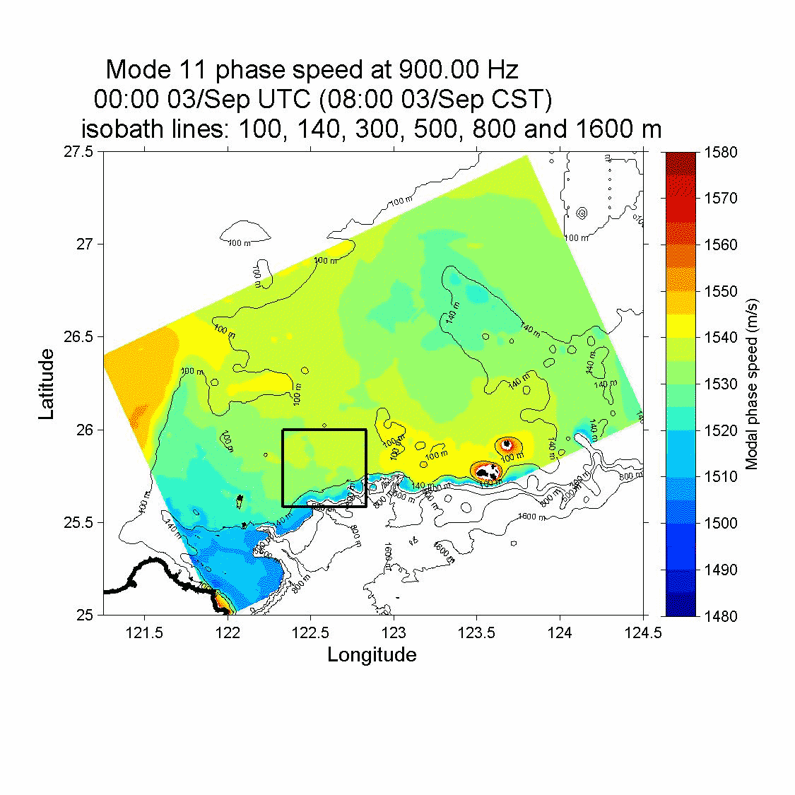
Sound frequencies: 600 Hz and 900 Hz; Normal Mode Calculation Domain Resolution: 800 m
Water column: Real-time MIT MSEAS system (4.5 km resolution)
Bathymetry: MIT bathymetry data creating from UNH 100 and 500 m resolution data and NCOR data.
Bottom: 20 m deep sediment layer on the top of a basement with sound speed (c) 1,800 m/s, density (ρ) 2.0 g/cm3 and attenuation coef. (α) 0.5 dB/λ.
The sediment type depends on the local water depth (WD): when WD < 140m a sand sediment is given (c: 1,562 m/s, ρ: 1.9 g/cm3, α: 0.9 dB/λ);
whereas when WD > 140m a muddy-sand sediment is given (c: 1,549 m/s, ρ: 1.488 g/cm3, α: 1.15 dB/λ)
This forecast is for predicting the acoustic modal variability due to water-column condition changes. The normal mode program KRAKEN is used to calculate the local vertical modes at each point on the grid. It should be noted that the sediment type depends on the local water depth, as suggested by P. Lermusiaux and J. Xu of MIT on their bottom sensitivity study using QPE Pilot Study data. This work is sponsored by the ONR.
| Sep 03 0000Z (Sep 03 0800CST): Snapshot Time-Series of the Estimated Modal Phase Speeds(every 3 hours) | ||||||||||||
|---|---|---|---|---|---|---|---|---|---|---|---|---|
| Click on any mode label for a full set of plots | ||||||||||||
|
||||||||||||
|
||||||||||||
| Return to the MSEAS: | |||
| QPE IOP09 real-time web page | QPE web page | Home page | |