

|
P.F.J. Lermusiaux, P.J. Haley, Jr., W.G. Leslie, T. Lolla, P. Lu, C. Mirabito, A. Phadnis, M. Ueckermann |
Massachusetts Institute of Technology
Mechanical Engineering Ocean Science and Engineering Cambridge, Massachusetts |
|
ONR 6.1 Supported Publications |
Previous ONR 6.1 Research |
Physical and Interdisciplinary Regional Ocean Dynamics and Modeling Systems
This research is concerned with the fundamental understanding and modeling of complex physical, acoustical and biogeochemical oceanic dynamics and processes. New mathematical models and computational methods are created, developed and utilized for: i) ocean predictions and dynamical diagnostics, ii) data assimilation and data-model comparisons, and, iii) optimization and control of autonomous ocean observation systems. The regional dynamics involves interactions of sub-mesoscale and mesoscale ocean processes in the littoral as well as effects from large-scale processes in ocean basins. Such interactions and feedbacks with scales smaller and larger than the mesoscale need be better quantified. The technical approach is rooted in the comparison and optimal combination of measurements and models via nonlinear data assimilation (DA), including the development of adaptive modeling and adaptive sampling schemes based on Error Subspace Statistical Estimation. Our research group is updating and renewing our previous approaches and computational schemes and systems. We will keep and modernize the strengths of our methods and codes, but we will also progressively utilize other ocean dynamical models, or parts thereof, and explore novel numerical systems.
The research topics that are specific to the present effort include:
- Three-dimensional (3D) acoustic modeling coupled with high-resolution 4D physics modeling
- Ocean modeling incubator: structured and unstructured grids; investigations and evaluations of the next generation of numerical schemes for physical, acoustical and biological dynamics
- Interactions of internal tides/waves and mixing processes with mesoscale dynamics, their high-resolution modeling and multi-scale diagnostics
- Lagrangian coherent structures and ocean features: their prediction, dynamics and assimilation
- Nonlinear DA and adaptive DA, including (super)-tidal constraints and assimilation
- Use of several ocean models, model uncertainty estimation, and multi-model fusion and DA
| Finite Volume Methods: A flexible, modular, and efficient framework for solving advection-diffusion-reaction equations, and the Boussinesq, Level Set, and Navier-Stokes equations in a rotating frame of reference was implemented in MATLAB. This framework allows for the rapid set up of new problems with complex stair-stepped geometry on a uniform, two-dimensional structured grid. The spatial discretization is first or second order in space, using a central differencing scheme for the diffusion operator, and either the Quadratic Upwind Interpolation for Convective Kinetics (QUICK) scheme, the Central Differencing Scheme (CDS), or the Upwind Wind (UW) scheme for advection. For the time discretizations, we use either a first or second order, backwards in time differencing scheme. The Boussinesq and Navier-Stokes equations are treated semi-implicitly, where the source terms, diffusion and pressure are treated implicitly, and the advection is treated explicitly. We use various different projection methods to enforce the divergence-free constraint. Using this framework allowed us to rapidly implement our Dynamically Orthogonal (DO) formulation of the Navier-Stokes and Boussinesq equations, test new algorithms for optimal path-planning, test novel data-assimilation schemes, and do comparative numerical studies. We have also used this framework for idealized studies of the Meridional Overturning Circulation. |
|
Discontinuous Galerkin Finite Element Methods:
We have further improved our 2D-in-space Discontinuous Galerkin Finite Element MATLAB framework (Ueckerman, 2009). New plotting,
analysis, meshing, and solver routines have been added. In particular, to address issues with numerical oscillations, a slope limiter was implemented for linear basis functions
(Hoteit et al., 2004), and a novel filtering approach was implemented for higher polynomial degree basis functions. Our approach is based on selectively applying an exponential
filter when the solution is non-smooth. Our smoothness indicator is a modification of that proposed in Mavriplis (1989). We tested both the slope-limiting and filtering approaches
by advecting tracers that have sharp or discontinuous jumps or fronts in the initial conditions. Using our framework, we completed a comprehensive numerical analyses, employing
standard and hybrid discontinuous Galerkin Finite Element Methods, on both straight and new curved elements (Ueckermann and Lermusiaux, 2010). Our analyses focused on
nutrient-phytoplankton-zooplankton dynamics under advection and diffusion within an ocean strait, in an idealized two-dimensional geometry. This allowed us to complete a
large number of sensitivity studies which we synthesized. For the dynamics, we investigated three biological regimes, one stable and two unstable with limit cycles. We also
examined interactions that are dominated by the biology, by the advection, or that are balanced. For these regimes and balances, we studied the sensitivity to multiple numerical
parameters including: quadrature-free and quadrature-based discretizations of the source terms; order of the spatial discretizations of advection and diffusion operators; order
of the temporal discretization in explicit schemes; and resolution of the spatial mesh, with and without curved boundary elements. We are now formulating a novel Hybrid Discontinous
Galerkin discretization for three-dimensional, non-hydrostatic, free surface ocean flows.
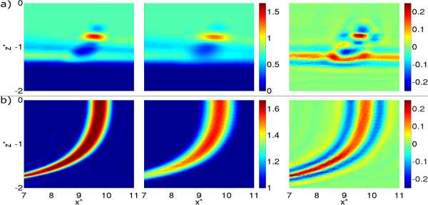
In our tests, the slope-limiter removed spurious numerical oscillations in tracer advection with sharp, discontinuous fronts. However, we noted additional diffusion in regions where the tracer fields were smooth. Our filtering approach, with an appropriately chosen strength, successfully removed spurious numerical oscillations for the same tests, but did not introduce additional diffusion where tracer fields were smooth (Ueckermann et. al., 2010). We obtained high-order accurate solutions of biological dynamics using our discontinuous Galerkin schemes (Fig. 1). We find that both quadrature-based and quadrature-free discretizations give accurate results in well-resolved regions, but the quadrature-based scheme has smaller errors in under-resolved regions. We show that low-order temporal discretizations allow rapidly growing numerical errors in biological fields. We find that if a spatial discretization (mesh resolution and polynomial degree) does not resolve the solution, oscillations due to discontinuities in tracer fields can be locally significant for both low and high-order discretizations. When the solution is sufficiently resolved, higher-order schemes on coarser grids perform better (higher accuracy, less dissipative) for the same cost than lower-order scheme on finer grids. This result applies to both passive and reactive tracers and is confirmed by quantitative analyses of truncation errors and smoothness of solution fields. To reduce oscillations in un-resolved regions, we develop a numerical filter that is active only when and where the solution is not smooth locally. Finally, our idealized simulations of biological patchiness (Fig. 2) reveal that higher-order numerical schemes can maintain patches for long-term integrations while lower order schemes are much too dissipative and cannot, even at very high resolutions. Implications for the use of simulations to better understand biological blooms, patchiness, and other nonlinear reactive dynamics in coastal regions with complex bathymetric features are considerable. |
|

|
Dynamically Orthogonal (DO) Evolution Equations for Flows with Uncertainty:
Building on our closed set of evolution equations for fields governed by Stochastic Partial Differential
Equations (SPDE) (Sapsis and Lermusiaux, 2009), we developed analytical criteria that instantaneously control and evolve the size of the subspace where uncertainty "lives".
Transient dynamics, sparse data and non-stationary statistics are typical in a large range of applications such as oceanic and atmospheric flows making essential to vary the
dimensionality of the stochastic subspace with time. We analyze the scaling of the computational cost with the stochastic dimensionality and show that unlike many stochastic
methods, the DO equations do not suffer from the curse of dimensionality. The new adaptive criteria for the variation of the stochastic dimensionality are based on i) stability
arguments and ii) Bayesian data analysis (Sapsis and Lermusiaux, 2010).
With this approach, the basis and dimensionality of the error subspace evolves according to the system SPDE and therefore fewer modes are required to capture most of the energy
compared to the POD or Polynomial-Chaos method that fixes the basis for flow field or stochastic coefficients a priori and can thus diverge. This is especially true for the case of
transient responses. While our approach is more computationally efficient than known existing methods, our first numerical solution algorithm required the inversion of S2 matrices for
solving the stochastic pressure, where S is the number of modes. By using a projection method, we solve for stochastic pseudo-pressures instead, thereby reducing the number of matrix
inversions to S. We proved that these stochastic pseudo-pressure correctly solve our equations, and that the statistics of the true stochastic pressures could be recovered by
post-processing. Our new algorithm drastically reduces the computational cost for cases with large number of modes.
The new numerical discretization was implemented in our flexible Finite Volume MATLAB framework (see above). We use: the second order in space version, the central differencing for the
diffusion operator, the QUICK scheme for advection by the mean fields, and the CDS for advection by the stochastic modes. For the time discretizations, we used semi-implicit
first-order backward differencing, where the diffusion and pressure are treated implicitly, and the advection explicitly.
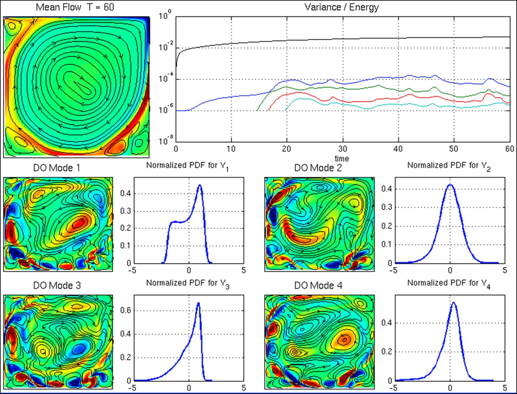
We found that the adaptive-size algorithm gave accurate results, and the new DO implementation was considerably more efficient (100-1000 time faster) than our first implementation. We apply the derived framework for the study of the statistical responses of the lid-driven cavity flow and "double gyre" circulation, which has elements of ocean, atmospheric and climate instability behaviors. In Figure 3 we present the mean flow (top - left) for the lid-driven cavity flow and for Reynolds number Re = 10000. For the considered Reynolds number, the flow is unstable causing a very small stochastic perturbation applied at the beginning to grow, leading to non-Gaussian statistics with strong spatial dependence. These properties are captured with our adaptive DO schemes. In Figure 4 we present the stochastic response of a double gyre flow driven by wind-stress forcing, constant in time and symmetric in space, in the presence of Coriolis acceleration. As in the previous case, instabilities lead to growth of an initially small stochastic perturbation. Our adaptive criteria allow for the efficient evolution of the stochastic subspace dimensionality. Moreover, we find that the mean flow preserve its symmetry properties while all the anti-symmetric part (which is due to the Coriolis terms) is captured by the stochastic modes. The bimodal symmetric structure of the probability density functions reveal the bi-stable states of the system, clearly illustrating that the system will "randomly" follow one of the two states in the bimodal distribution. |
|
 |
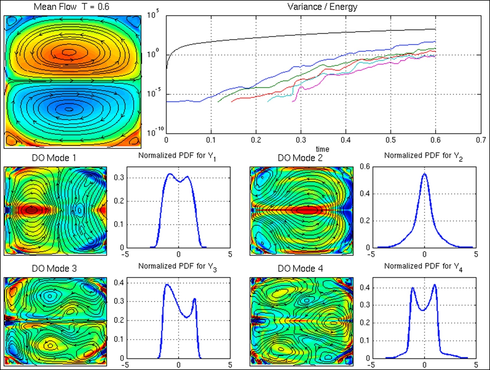 |
| Figure 3: Stochastic response of the lid-driven cavity flow for Re = 10000. The mean flow and the first four DO modes are shown in terms of their vorticity and streamlines. The variance and energy of the modes and mean flow, respectively, are shown as well as the one dimensiona l marginal for the four stochastic coefficients. | Figure 4: Stochastic response of the forced double gyre flow for Re = 10000. The mean flow and the first four DO modes are shown in terms of their vorticity and streamlines. The variance and energy of the modes and mean flow, respectively, are shown as well as the one dimensional marginal for the four stochastic coefficients. |
|
Optimal Path Planning for Vehicle Swarms in Time-Varying Uncertain Velocity Fields:
A new method for calculating optimal vehicle paths and headings was formulated, without any
limitation on the strength of currents. Using a level-set representation, a "wavefront" of possible optimal vehicle positions is evolved in time. By saving the shape of the
wavefront at each time instance, along with the corresponding currents, the optimal path is generated through a backward integration method. A number of tests were examined
using specified velocity fields. First, we employed analytical and canonical ocean flows such as "uniform", "straight jet", "meandering jet" and "ocean eddy" flows.
Our new method was also used with more complex ocean fields such as stochastic two-dimensional double-gyre flows. Using our CFD codes (see above), an idealized 2D wind-driven ocean
circulation field was used to evolve the level sets. Here, optimal paths in strong complex currents are calculated. The magnitude of the uncertainty on the "wavefront", computed
using our DO field equations, was also extracted at each time instance. Examples of goals specified were: sampling as far north as possible; and sampling the south-west corner of the
domain from a specified starting position.
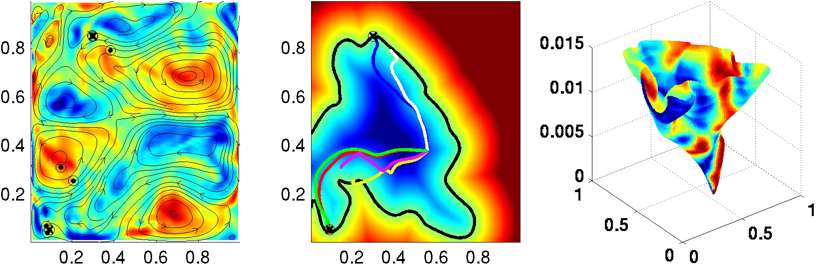
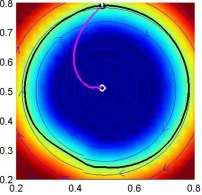
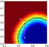
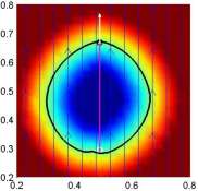
Results using idealized canonical flow fields are illustrated in Figs. 5a-5d. Such canonical flows could be very useful as rules-of-thumb for naval operations. The results for an example of complex flows are illustrated in Figure 6. The targets are i) sampling as far north as possible, and, ii) sampling the south-west corner of the domain, in both cases from a specified starting position. This figure shows that the optimally planned paths are the ones that reach the desired targets the fastest. Trajectories chosen assuming no flow-field do not reach their targets, and do not exist on the wavefront of best possible paths (e.g. see the magenta path). The green path illustrates the plan of a "smart oceanographer". After studying the flow field, it was assigned a due west heading for a certain amount of time, followed by a due south heading. The transition time between headings was determined by looking at the trajectory of the optimally planned path and flow fields. While this insightfully guessed green path does approach the target point, the red path still gets first to the target. This reveals that, though a very good guess could reach the desired targets in a quasi-optimal time, the calculated optimal path is still superior and is computed autonomously. We also show the evolution of the zero-level set superimposed with the magnitude of the local uncertainty. Future work includes finding paths that optimally utilize or reduce flow uncertainties. Another next step would be to predict the uncertainty of the level-sets themselves. |
|||||
|
 |
||||
| Figure 5: Results of optimal path planning in idealized canonical flow-fields. Each plot shows the level set function with the zero level-set highlighted in black. The path is shown in magenta; the starting position is indicated by the white circle, and the ending position by the black circle. The instantaneous vehicle heading is shown in white. The flow-fields used are a) clock-wise circular eddy, b) strong front with parabolic profile, c) uniform flow to east, and d) uniform flow north. | Figure 6: Results of optimal path planning in complex, uncertain flow-field. (Left) The mean flow vorticity plotted in color with streamlines superimposed. Vehicle positions are indicated by open circles with solid dots, and targets are indicated by open circles with crosses. (Center) The level set function, with the zero-level set highlighted. The red and blue paths are the results from optimal path-planning. The magenta and white paths are chosen assuming no flow-field, the yellow path is a poor guess and the green path is a good guess. (Right) The evolution of the zero level set over time, colored by the uncertainty of the flow-field. | ||||

|
Data Assimilation using Gaussian Mixtures, Minimum Divergence Filters and DO Equations:
Our DO field equations (Sapsis and Lermusiaux, 2009) allow efficient evolutions of multi-dimensional
probability distributions described by SPDEs. Studying these probabilities, we find that at any instant, for sufficiently nonlinear dynamics, both marginal and joint distributions of the
random DO coefficients exhibit severe multi-modalities. Hence, we are developing new data assimilation schemes that use these probabilities as inputs and respect the non-Gaussian structure
that can arise in reality.
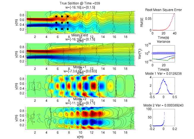
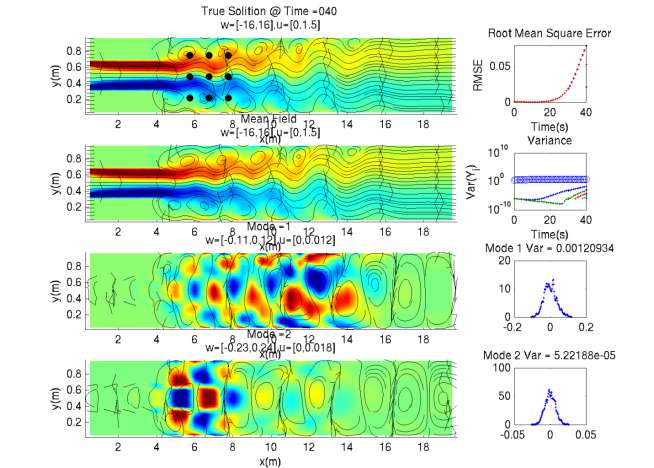
Traditional assimilation schemes partially retain the assumptions of linearity and Gaussianity in the analysis step, as in the Kalman Filter, and thus typically do not use information beyond the first two moments of the ensemble distribution. Consequently, much of the non-Gaussian structure may be lost during the analysis. One new scheme we are investigating is based on approximating the prior distribution by a Gaussian mixture. This is determined using the Expectation-Maximization (EM) algorithm and tested for optimality using the Bayesian Information Criterion. We consequently perform the analysis step by implementing update for each Gaussian mixture component, weighted by its likelihood as determined by the EM-algorithm. In the limit of large mixture complexity and ensemble members, this method may be shown to reproduce the Bayesian update. The Minimum Divergence Filter is an assimilation scheme which uses general background probability density functions. The framework proves particularly useful in cases where the background distribution exhibits multimodal behavior, e.g. as for the Kuroshio. At the analysis step, the prior distribution is determined as that which minimizes the Kullback-Leibler (K-L) divergence among a set of distributions consistent with specific moments of the background distribution. We have implemented the scheme in a tracking scenario using the "Double Well Diffusion Experiment", assuming a Gaussian Mixture. Work is underway to extend the schemes to more complex cases. Using our 2D Finite Volume codes, we tested of our new DA schemes on simple double-well problems as well as on several 2D flows. One 2D flow example is a sudden expansion in a pipe which forms re-circulation eddies and instabilities similar to those of ocean jets. Figs. 7a and 7b plot snapshots of the results at two arbitrary, but adjacent, time instants. The transition in time, during which data is assimilated, clearly shows the ability of the new filter to capture the true solution via appropriate assimilation of the limited data. Fig. 8 further shows how the new DA scheme captures the non-Gaussian structure of the probability density function. Preliminary results show improvements over DA schemes using Gaussian-based analyses, including the Ensemble Kalman Filter. |
|
 |
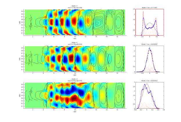 |
| Figure 7: (a) Data assimilation using Gaussian Mixtures and the DO equations, for a sudden expansion test case. The top-left figure shows the true solution that we wish to approximate. Then, the prior mean field estimate and its first two prior DO uncertainty modes are shown, as well as the two distributions for the latter. We also give the energy of the mean field as well as the variances of each of the marginal distributions. Observations are simulated to occur at the nine black dots: the data are the u- and v- velocities, measured every ten time units. (b) Posterior estimate following assimilation of noisy observations using the new DA scheme. Comparing of this updated mean field with the prior mean field (see Fig 7a), we've managed to accurately capture the structure of the true solution using a new DA scheme and the set of noisy observations. In the top-right plot, we further show the root mean square error (RMSE) of the approximation compared with the true solution. In blue, we plot the RMSE for the Gaussian Mixture Modeling DA scheme. This is compared with the results produced using the Ensemble Kalman Filter in red. Clearly, at time step 40, the new scheme outperforms the Ensemble Kalman Filter. | Figure 8. Probability density representations using DO equations and Gaussian Mixtures, for a sudden expansion test case. Shown are modes 1-3 and their respective random coefficients at a given time instant. Of particular interest is the top-right plot (highlighted in red) which shows the marginal distribution of the random coefficient of the first mode. The blue-dotted curve is the kernel density approximation to the particle distribution, clearly exhibiting non-Gaussian structure. The red-solid curve shows the Gaussian mixture approximation, which is a weighted sum of the red-dotted Gaussian mixture components, determined using the EM-algorithm. The black curve shows the approximation to the particle distribution using the Ensemble Kalman Filter. Clearly, the Gaussian mixture captures the non-Gaussian structure while the Ensemble Kalman Filter does not, which affects the analysis step. |
|
Ocean Dynamics, Modeling and Assimilation:
In Haley and Lermusiaux (2010) we derived conservative time-dependent structured discretizations and two-way embedded (nested) schemes for
multiscale ocean dynamics governed by primitive-equations (PEs) with a nonlinear free surface. We first provided an implicit time-stepping algorithm for the nonlinear free surface
PEs and then derived a consistent time-dependent spatial discretization with a generalized vertical grid. This leads to a novel time-dependent finite volume formulation for structured
grids on spherical or Cartesian coordinates, second order in time and space, which preserves mass and tracers in the presence of a time-varying free surface. We then introduced the
concept of 2-way nesting, implicit in space and time, which exchanges all of the updated fields' values across grids, as soon as they become available. A class of such powerful nesting
schemes applicable to telescoping grids of PE models with a nonlinear free surface was derived. The schemes mainly differed in the fine-to-coarse scale transfers and in the interpolations
and numerical filtering, specifically for the barotropic velocity and surface pressure components of the two-way exchanges. We completed a theoretical truncation error analysis of the
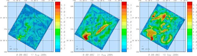
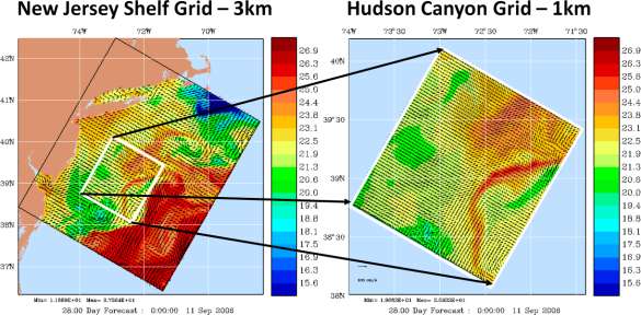
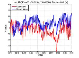
A manuscript on the oceanographic and atmospheric conditions on the continental shelf north of the Monterey Bay during August 2006 was submitted (Ramp et al, 2011), showing that multiscale 2-way nested modeling systems were most accurate for the region allowing for example to capture some of the cross-shelf transports. A review of the multiple scales and features occurring in the California Current System was submitted (Gangopadhyay et al, 2011), including the development of a Feature-Oriented Regional Modeling System for the region. A special edition of Ocean dynamics on multi-scale modeling of coastal, shelf and global ocean dynamics was completed (Deleersnijder et al, 2010). A publication on "Many Task Computing" for multidisciplinary real-time uncertainty prediction and data assimilation was written and accepted (Evangelinos et al., 2010) and earlier results published (Evangelinos et al., 2009). The dynamic coupling of models and measurements for a Dynamic Data-Driven Application System (DDDAS) is described based on examples in Massachusetts Bay, and Monterey Bay and the California Current System (Patrikalakis et al., 2009). Our study of 2-way nesting schemes showed that for nesting with free surfaces, the most accurate schemes are those with the strongest implicit couplings among grids, especially for velocity (Haley and Lermusiaux, 2010). For the simulations studied, the scheme with the least amount of fine grid feedback (Fig. 9) had differences between the barotropic velocity estimates of O(10) cm/s, with the structures of the difference field organized on the (sub)mesoscale. Conversely, the scheme with the most feedback (Fig. 10) had the smallest discrepancies, much smaller than 1 cm/s except near steep topography or strong dynamical gradients where differences reach 1 cm/s: the finer grid is needed there to represent this variability. With our theoretical truncation error analysis, we revealed the benefits of additional feedback from the fine to coarse domains. We proved that coarse domain estimates which are made up from averages of fine domain estimates retain the truncation error of the fine grid. Even for a second order scheme with only a 3:1 refinement, this equates to an order of magnitude reduction in the truncation error at these coarse domain points. A corollary of this analysis is that the improvement from the fine grid feedback can be guaranteed only if the feedback algorithm (in our case volume-averaging) has at least the same order of accuracy as that of the overall discretization. In our three realistic simulations, we resolved large domains with multiscale dynamics, including steep bathymetries and strong tidal flows in shallow seas. In each case, we found that without our new discrete PE model, or without nested grids, predictions do not match the ocean data. Specifically, in the middle Atlantic Bight (Fig. 11), we compared nested estimates to mooring data not assimilated in simulations (Fig. 12). Using twin experiments between a 3km resolution "stand-alone" domain and the same domain with a two-way nested 1km resolution domain, we showed that the addition of the nested sub-domain removes large biases and RMSEs, O(10-15) cm/s, in the model velocities when compared to the mooring data. The 2-way nesting scheme is found especially needed during tropical storm Ernesto. It is also required for future studies of internal tide propagation. In our study of the multiscale dynamics in the Philipines (Lermusiaux et al, 2011), our oceanographic findings include: the biogeochemical features forecast in real-time, the multiscale circulation features and their characterization, the evolution of flow fields within three major straits, the estimation of transports to and from the Sulu Sea and the corresponding balances, and finally, an investigation of multiscale mechanisms involved in the formation of the deep Sulu Sea water. |
|
 |
 |
| Figure 9: Baseline nesting (least implicit feedback). Vector differences between barotropic velocity in coarse and fine domains plotted in the fine domain for 00Z on 17 Aug., 31 Aug., and 18 Sep. (overlaid on magnitude of barotropic velocity differences). | Figure 10: Fully implicit nesting scheme (most implicit feedback). Vector differences between barotropic velocity in coarse and fine domains plotted in the fine domain for 00Z on 17 Aug., 31 Aug., and 18 Sep. (overlain on magnitude of barotropic velocity difference). Velocity differences are small with intermittent misfits at the shelfbreak. |
 |
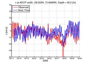 |
| Figure 11: Surface temperature, overlaid with surface velocity vectors, for 0000Z on 11 Sep 2006 in the fully implicit two-way nested New Jersey Shelf and Hudson Canyon domains. Note the filaments which were spun off of the shelfbreak front during the relaxation period follow ing the passage of tropical storm Ernesto (31 Aug - 1 Sep, 2006). | Figure 12: Hourly meridional velocities (v) at 68m depth at the location of mooring SW30, as measured by the moored ADCP (red curves) and as estimated by re-analysis simulations (blue curves) with atmospheric and barotropic tidal forcing. No mooring data are assimilated. (a) Comparing mooring velocities against velocity estimates from a 3km simulation without nesting ("Stand Alone"). (b) Comparing mooring velocities against velocity estimates from a 2-way nested simulation. Our new nesting scheme removes an O(15 cm/s) bias, as averaged during Aug 22-Sep 09. Notice that this bias reaches O(30 cm/s) during the Tropical Storm Ernesto. |
Modeling Uncertainty Generation: Understanding how uncertainties are generated in ocean models is very important for better predictions. We started developing for the MSEAS PE model a mathematically rigorous and computationally tractable way to diagnose the intrinsic source of uncertainties, based on a concise physical law recently discovered on entropy evolution (Liang, 2008). This diagnostic quantity has been named local entropy generation (LEG). We have tested the new approach with the data set and simulations for the SW06 sea experiment. The results agree with physical intuition. We also tested it against model scheme changes. This approach is expected to provide an objective way of ocean model assessment. Modeling Uncertainty Generation: We find that an ocean model can be objectively assessed in terms of uncertainty generation through computing a diagnostic quantity that we namely local entropy generation (LEG). An explicit formula for the MSEAS model was derived, and made computationally tractable. Tests have been successfully performed with a dataset acquired from the sea exercise SW06.
Multiscale Energy and Vorticity Analysis (MS-EVA): In order to conduct dynamical studies for our real-time sea exercises, the localized multiscale energy and vorticity analysis (MS-EVA) of Liang and Robinson (2005) and multiscale window transform (Liang and Anderson, 2007) have been been adapted to the MSEAS PE model. MS-EVA diagnostics were run for the SW06 dataset. Multiscale window transforms were performed, and reconstructions made for all the field variables. We are studying the dynamical processes underlying the observed complicated shelf-slope frontal variabilities.
Acoustic Predictions: Lin et al. (2010) utilizes a novel empirical orthogonal function (EOF) fitting technique to combine time-varying data profiles from multiple sources, including our model estimates, into sound speed profiles indicative of conditions at a single site. The resulting profiles have been used in acoustics propagation modeling endeavors and have improved acoustic data-model comparisons.
Adaptive Sampling: A new manuscript on the quantitative planning of the paths of AUVs combining Mixed Integer Linear Programming (MILP) with ESSE forecasts of data impacts has been further improved (Yilmaz and Lermusiaux, 2010). Schemes for adaptive sampling based on genetic algorithms have been further evaluated (manuscript in prep). Multiscale modeling with tidal forcing was used to guide automated sensor networks (Schofield et al, 2010).
| Top of page |